Friston's Free Energy Principle Explained (part 1)

The goal of this series of posts is to provide a friendly but rigorous guide to some of the key ideas underlying Karl Friston’s Free Energy Principle (henceforth: FEP). I will provide as much background as possible, and sprinkle in the intuition-pumps I find most helpful. I want this to be a technical guide, so we won’t shy away from any math¹. Your reward for making it to the end will be a deep understanding of the core pieces of the Free Energy principle, the ability to explain it to an interested friend in plain english, and the ability to implement a simulation of Active Inference under the Free Energy Principle in Python! But before we get to the Python, we need to lay the groundwork…

By the end of this post you will understand:

• Bayesian inference
• ‘Phenotype’ as a set of viable states
• Entropy and expected surprise
• Kullback-Liebler Divergence
• Recognition- and Generative-densities
• The derivation of the ‘free energy’ term

Introduction

Karl Friston’s Free Energy Principle has fascinated and baffled me since I first heard about it in a SlateStarCodex blog post². Ever since, I’ve spent a good chunk of my spare time trying to understand the ideas and context that underpin the theory. Friston’s work is notoriously difficult to understand, something which Friston himself (and definitely the people who read his work) acknowledge with a wry shrug³. This comes down to a few things:

• the maths itself is fairly daunting and Friston’s notation can be opaque until you get used to it. But, I’ll show you in this article that it’s not impenetrable and is well worth understanding!
• the fields that Friston draws on to derive the FEP are diverse and any given person is unlikely to have studied them all⁴. I happen to think this is what’s most exciting about the FEP, because it provides an excuse to learn more about:
  • Statistical Mechanics, especially non-equilibrium stat-mech
  • Reinforcement Learning
  • Neuroscience and Predictive Coding
  • Dynamic systems and (stochastic) differential equations
  • Information theory
  • Variational inference methods
  • Path-integral formulations and the Principle of Least Action
  • Embodied cognition
  • Bayesian inference, action under uncertainty
  • Clinical psychiatry and computational corelates of pyschopathology

For this post, don’t worry about that list, as I’ll introduce concepts as we need them!

To begin, let’s look at some motivating ideas, which we’ll keep coming back to, with more and more formalism to back them up.

You: a thing in the world

You are a thing (fully enlightened Buddhists with no sense-of-self don’t @me yet please, it’s just a starting point) and you live in a world which you do not fully understand (or at-least, it should feel that way, if you’re paying any attention to how crazy things are right now).

You get a constant stream of new information through your senses, and your brain somehow needs to use this information-deluge to do things like make exceptional scrambled eggs, renew your driver’s licence, floss your teeth, and other crucial survival-skills.

Eye on the (causal) prize

Our first big insight into the FEP is that if you want to keep doing the survival thing, you should care not about the sense data itself, but about the stuff out there that causes it - you need to keep your eye on the causal prize! The sense data is just receptors firing more or less often. What matters is that you have receptors that reliably fire in a pattern that tells you useful things like:

• there’s a tiger there and she looks pissed
• it smells like chocolate cookies have just come out the oven, so you might get fed soon
• the molten chocolate cookie you just inhaled is scalding your oesophagus and causing long-term scarring

So your sense-data isn’t random - it has external causes - but it’s not perfectly reliable either. It’s a noisy connection, and ambiguity abounds:

• is that a burglar standing in the corner of your dark room, or did someone leave a coat hanging on your hatstand?
• is that the rustling of the wind in the leaves, or another, even scarier tiger stalking you?
• is the pressure of your ‘deep-tissue sports-massage’ a welcome relief from stiffness, or categorical proof that your masseuse is a sadist?

Macro-stable, micro-random

In the time you read all of the above, you breathed several times, each of your cells used some ATP, some cells died or were phagocytosed, the state of your brain changed and a bunch of different neurons fired, and yet You are still a thing in the world. From this I infer that you did not suddenly dissolve into an unremarkable puddle of goo in the preceding 30 seconds. This is our second big insight into the FEP: as a system, many little things can change (you are dynamic), but you must keep yourself tightly bound into a larger pattern - you can be micro-random but must be macro-stable!. Friston often refers to this as possessing an ‘attracting set’ - a set of states that all of your bizarre chemical processes can wiggle around in and between, but not out of.

There are lots of ways you could configure all of the atoms that currently constitute ‘you’. Unfortunately, the vast majority are unworkable, probably because the most likely arrangement of those atoms is spread in a thin mist somewhere between here and Neptune. The small subset of all possible ways to configure yourself that keeps you ‘you’ is your phenotype, and homeostasis is basically the process of keeping yourself in those states through feedback and self-regulation. To survive long-term, you need to have a high probability of occupying those states that are compatible with life (and a low probability of becoming a thin mist somewhere between here and Neptune)

Let’s make a concrete example out of temperature…

It’s getting hot in here (and that’s surprising)

Your body keeps itself near 37 degrees (Celsius), all the time⁵

If you were suddenly to sense a temperature of 800 degrees, that would be surprising. And bad. As an organism, 800 degrees is not compatible with your continued existence, and is not something your phenotype is equipped to deal with. In this sense, your body is implicitly making a claim that there is a low probability of you experiencing 800 degree heat, because if that were not the case, you would have a different body. Since 37 degrees seems cosy enough, your body itself is an implicit expectation of a high probability of sensing that temperature⁶.

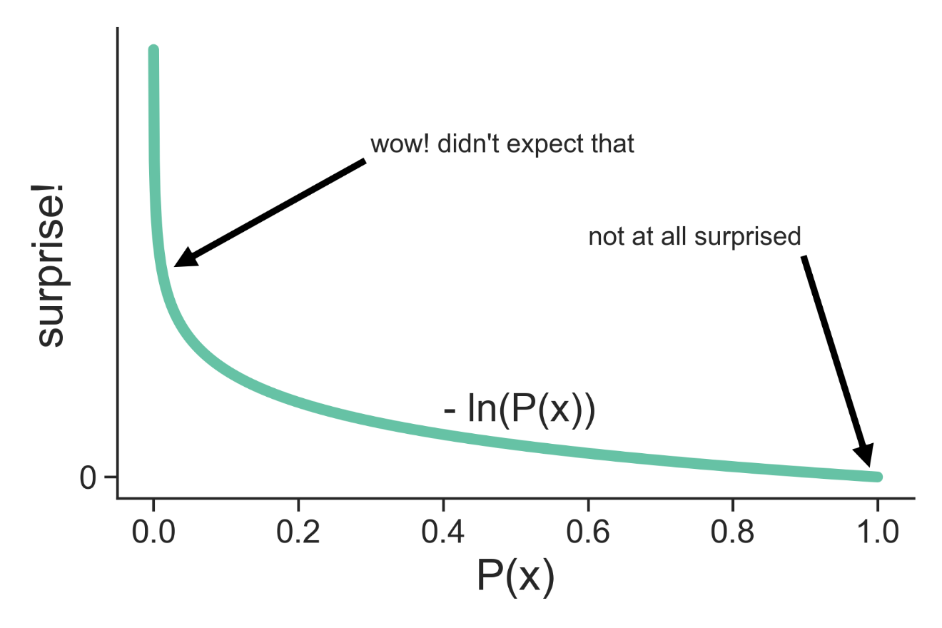
So your evolved biology ‘expects’ 37 degrees , and when it doesn’t get it it’s surprised. This ‘surprisal’ is actually a formal term from information theory, where we quantify the amount of surprise as the negative natural logarithm of the probability of the observed outcome:

$$- \ln P(X = x)$$

All this is saying is that the lower the probability we expect for an event, the more surprised we should be if we do in-fact observe that event, and conversely, if we think there is a high probability of an event happening, we should not be very surprised to see it occur. If you enter the lottery, and I tell you you’ve won, you’d be really really surprised, because you know the probability of that is small. If I tell you you’ve lost, you’re not really surprised at all, as that was always the likely outcome.

Let’s drill a little deeper into this business of sensing something and - on the basis of that sensation - forming accurate beliefs about the temperature of the environment and your body. It’s worth saying: you don’t have a nice digital-thermometer organ attached somewhere to your body which your brain can just look at. You have millions of tiny sensory receptors, which fire because of the energetic bumping and jostling of atoms hitting the receptor. For a temperature receptor, when it’s hotter, the atoms hitting it have a higher average energy, which makes it more likely that the neuron the receptor is attached to is depolarised and fires an action potential (“spikes”). We can roughly reason that in hotter environments, our temperature receptors are firing more often (but only on average - it’s still a “noisy” signal), and so maybe if our brain counted the number of spikes in a certain time, it could learn a mapping from the state of the sensory data it receives to the probable temperature of the environment.

All Reality is Virtual Reality

This gives us our third big clue about the FEP: we don’t directly experience the environment, only the noisy sensations that correlate with it - we’re one layer removed from the world, exploring the virtual reality of our sense data and inferring things about the reality behind it. This is really the jumping off point for the FEP: as an organism, we need to minimise our surprisal (we don’t want to find ourselves in 800 degree heat, and do want to find ourselves at 37 degrees, with high probability), but we only have access to our noisy sense data, and we don’t know what causally determines our temperature in the environment.

Getting Bayesian

As organisms, we want to update our beliefs about the true state of the environment, given some sense data as evidence. That’s right, it’s time for⁷

(obligatory link to Yudkowsky on Bayes Theorem. If this is new, read this now)

Bayes theorem tells us the optimal way to update our beliefs given some new evidence. Doing this is sometimes called Bayesian inference, or Bayesian updating, or - controversially - as “not making up your beliefs”.

A brief note on integral notation: I will often write integrals like this: $ \ \int_{}^{}{dx\ f(x)}$ with the $dx$ at the front of the integral. If you're used to seeing it at the back, like this: $ \ \int_{}^{} f(x)\ dx$ don't freak out, they're exactly the same. Also, I'm going to leave the bounds of integration out for now. We can add them in if we need them later

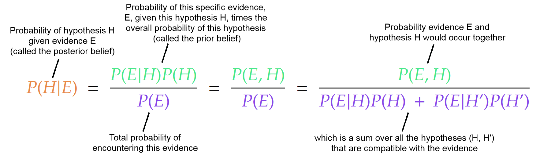
What we want is to update our belief about the state of the environmental temperature, given our current sensory data. Let’s write the prior probability that our temperature is 37º as $P(T)$, and the probability that we receive 40 incoming neural impulses in a given time as $P(S)$. We want to know the updated probability that our temperature is 37º, given that we sense 40 neural spikes:

$$P(T|S)$$

So our hypothesis is that the temperature is 37 degrees, and the evidence we’re using to evaluate it is the 40 spikes we received in the last few seconds.

$$P\left( T \middle| S \right) = \frac{P\left( S \middle| T \right)P\left( T \right)}{\blue{P(S)}}$$

The $\blue{P(S)}$ term seems to cause trouble, so I'm going to spend a little extra time explaining it here, using the example of modelling the weather today based on yesterday's weather: The probability of it being sunny today, $P(\text{Sunny})$ can be thought of as the sum of the two possibilities - it could be sunny today, given that yesterday was sunny, or it could be sunny, given that yesterday was **not** sunny: $$P(\text{Sunny}) =\\ P(\text{Sunny}|\text{sun yesterday})P(\text{sun yesterday}) +\\ P(\text{Sunny}|\text{no sun yesterday})P(\text{no sun yesterday})$$ Instead of the sum of these two complementary outcomes, we could sum over each different possibility: $$P(\text{Sunny}) =\\ P(\text{Sunny}|\text{sun})P(\text{sun}) +\\ P(\text{Sunny}|\text{rain})P(\text{rain}) +\\ P(\text{Sunny|snow})P(\text{snow}) +\\ P(\text{Sunny|tornado})P(\text{tornado}) + ...$$ Which we can compress as a sum over each possible weather state: $$P(\text{Sunny}) = \sum_{weather}{P(\text{Sunny|weather})P(\text{weather})}$$

Based on the box above, we want to write $P(S)$ like this:

$$\blue{P(S) = \sum_{i}{P(S|T_i)P(T_i)}}$$

but we must remember that, unlike our discrete weather states above, temperature is a continuous variable (it’s just a real number, which can take any value). Therefore, we replace the sum over states with an integral over all temperature values:

$$P\left( T \middle| S \right) = \frac{P\left( S \middle| T \right)P\left( T \right)}{\blue{\int_{}^{}{P\left( S \middle| T \right)P\left( T \right)\text{dT}}}}$$

And there you have it. All you need to do to perfectly understand the world is know the probability of experiencing some sensory data given a particular environmental state, and evaluate the probability of experiencing that sensory data under every possible hypothetical temperature. Very simple stuff!

Okay, so that integral is intractable, which is formal mathematical language for ‘Wolfram Alpha can’t compute it’. This is a problem for the FEP, and much of the rest of our effort will go into getting around that integral. When we can’t get an exact result, we turn to approximate methods. We’re going to manipulate our equation above until it’s in a form that allows us to do approximate Bayesian inference.

Approximating your posterior

We want to find the posterior probability (the probability we get after applying a Bayesian update) that:

$$P(T=37|S)$$

It would really help us control our body temperature if we understood the causal influences determining it. Intuitively, we want a world-model that predicts that if we move closer to a heat-source, we’ll get sensory data that tells us we’re getting hotter.

The internal model that encodes how we expect our sense data to correlate with our environmental states is called a Generative Model, and is referred to by Friston as the G-density. Our G-density tells us the joint probability of experiencing some sense data and a corresponding environmental state: $P(T,S)$

You can imagine this as a big table that assigns a probability to each possible pair of values. A good model in this case would assign a high probability to the combination:

$$P(\text{high temp, lots of spikes})$$

and a low probability to things like:

$$P(\text{high temp, few spikes})$$

We will also want a function that represents our current ‘best-guess’ as to the causes of our sensory input, which we’ll call the R-density (for Recognition): $q(T)$

This is just a probability distribution over the state of the environment, and we’re using $q$ instead of $p$ to remind us that it’s a distribution we’re guessing at.

We now need another fancy piece of information theory: the Kullback-Liebler (KL) Divergence⁸

The KL Divergence just tells us how different two different probability distributions are:

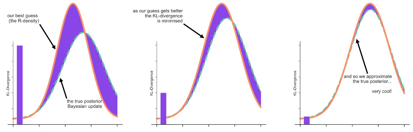
We want the KL divergence because we want to know how close or far away our best guess is to the true posterior belief if we could compute that ugly integral

We write the KL-divergence between our guess $q(T)$ about the environment and the optimal posterior belief about the environment from Baye’s theorem:

$$D_{\text{KL}}(q(T)||P(T|S))\ = \ \int_{}^{}{\text{dT}\ q( T )\ln\frac{q\left( T \right)}{P\left( T \middle| S \right)}}$$

which we rearrange using the property of the logarithm to:

$$= \ \int_{}^{}{dT\ q(T) \lbrack \ln{q(T)\ - \ \ln P(T|S)\rbrack}}$$

Now, any R-density (that is, any $q(T)$) which minimises this KL divergence, must be a good approximation of our true posterior. The only problem is that we don’t know the true posterior (that’s the thing we’re trying to work out in the first place), and so can’t simply guess a $q(T)$ to see if it minimises the KL Divergence, because we don’t know what we’re comparing it to.

To get around this, we’ll rewrite the true posterior

$$\orange{P(T|S)}$$

using some pretty basic probability theory identities:

$$\orange{P( T | S )} = \frac{\blue{P( S | T )P( T )}}{\purple{P( S )}}$$ $$\blue{P( T,S ) = P( S | T )P( T )}$$ $$\therefore \orange{P( T | S )} = \frac{\blue{P( T,S )}}{\purple{P( S )}}$$

If we take the natural log of both sides:

$$\ln{\orange{P \left( T \middle| S \right)}} = \ln{\frac{\blue{P\left( T,S \right)}}{\purple{P\left( S \right)}} = \ln{\blue{P\left( T,S \right)}} - \ln{\purple{P \left( S \right)}}}$$

Plugging this expression for $P(T | S)$ into our KL Divergence we get:

$$D_{\text{KL}}(q(T)||\orange{P(T|S)})\ = \int_{}^{}{dT\ q(T) \lbrack \ \ln{q\left( T \right) - \ln{\blue{P\left( T,S \right)} + \ln{\purple{P\left( S \right)}}}}}\rbrack$$

Combining the first two $\ln$ terms:

$$D_{\text{KL}}(q(T)||\orange{P(T|S)})\ = \int_{}^{}{dT\ q(T) \lbrack \ln{\frac{q\left( T \right)}{\blue{P( T,S)}}\ + \ \ln{\purple{P\left( S \right)}}\ }}\rbrack$$

Something you may notice about this is that we now have our KL divergence in terms of only our R-density, $q(T)$, and our G-density, $P(T,S)$, plus a ‘surprisal’ term $\ln P(S)$. This looks like progress! Remember, our R density is just our current best guess about the true state of the environment, the G-density is our internal model of how sensory data and environmental states correlate, and surprisal tells us how unexpected some data was!

We can pull the $\ln P(S)$ out from under the integral because integration is linear we’re integrating over $dT$ and so $\ln P(S)$ acts like a constant (it’s just a number):

$$D_{\text{KL}}(q(T)||P(T|S))\ = \int_{}^{}{\text{dT}\ q(T)\ \ln{\frac{q\left( T \right)}{\blue{P( T,S )}}\ }} + \ln{\purple{P(S)}}\int_{}^{}{dT\ q(T)}$$

Furthermore, we have the requirement that

$$\green{\int_{}^{}{\text{dT}\ q \left( T \right) = 1}}$$

which just says that the total probability must add to 1. Using this, we get:

$$D_{\text{KL}}(q(T)||P(T|S))\ = \pink{\int_{}^{} \text{dT}\left\lbrack q \left( T \right)\ln{\frac{q\left( T \right)}{\blue{P\left( T,S \right)}}\ } \right\rbrack} + \ln{\purple{P\left( S \right)} \times \green{1}}$$

Now, we define:

$$F\ \equiv \pink{\int_{}^{}\text{dT}\left\lbrack q\left( T \right)\ln{\frac{q\left( T \right)}{\blue{P\left( T,S \right)}}\ } \right\rbrack}$$

Giving us:

$$D_{\text{KL}}(q(T)||P\left( T \middle| S \right)) = F + \ln{P(S})$$

If you haven’t guessed already, the F we defined above is ‘free energy’!!. Now we have a key result in the Free Energy literature, one which Friston refers to all the time:

Free energy is an upper bound on surprisal!

You can see this if I tell you that the KL divergence has the property that it is always greater than or equal to zero:

$$D_{\text{KL}}(q(T)||P\left( T \middle| S \right)) \geq 0$$ $$\Rightarrow F\ + \ \ln{P\left( S \right)} \geq \ 0$$ $$F\ \geq \ - \ln{P(S)}$$

Free energy is the surprisal an organism experiences upon sampling some data, given a generative model.

More specifically, free energy is the surprisal an organism experiences upon sampling some data, given a generative model. If you’re up for it, you should try matching those words to the parts of the equations that encode them! I’ll even put the full equation right here in-front of you, with no distracting colours:

$$F\ \geq \ - \ln{P(S)}$$ $$\int_{}^{}\text{dT}\left\lbrack q\left( T \right)\ln{\frac{q\left( T \right)}{P\left( T,S \right)}\ } \right\rbrack \geq - \ln P(S)$$

So far, we have found that this quantity ‘free energy’ is an upper bound on surprisal, and we notice that minimising it means we are approximating the true posterior

$$P(T|S)$$

Another form of the free energy:

We’re going to need to massage this equation for F a bit more to see if something useful pops out.

Again, using the linearity of integration and the properties of the logarithm, we have:

$$F\ \equiv \int_{}^{}\text{dT}\left\lbrack \\ q\left( T \right)\ln{\frac{q\left( T \right)}{P\left( T,S \right)}\ } \right\rbrack$$ $$F\ = \ \int_{}^{}\text{dT}{\ q(T)\ \ln{q(T)\ \ } -}\int_{}^{}{\text{dT}\ q(T)\ln{P(T,S)}}$$

From statistics, we say that the expected value (or average) of a Random Variable $X$ is the sum over all values that variable can take, times the probability it takes that value:

$$E\lbrack X\rbrack\ = \ \sum_{i}^{}{x_{i}P(X=x_{i})}$$

If you need a sanity check, let's compute this for a fair 6-sided die. The probability for each face landing up is $1/6$ The values our random variable $X$ can take are $X = \{1,2,3,4,5,6\}$ $$E[X] = \sum_{x=1}^{6}\frac{1}{6}x = 3.5$$ which is indeed the correct average value for our die 🎲

Replacing the sum with an integral in the continuous case:

$$\displaystyle \operatorname {E} [X]=\int _{\mathbb {R} }xP(x)\,dx$$

We also have the entropy of a system (you should convince yourself that this is the “expected value” of the surprise $-\ln P(x)$):

$$\mathrm {H} (X)=-\sum _{i=1}^{n}{\mathrm {P} (x_{i})\log \mathrm {P} (x_{i}})$$

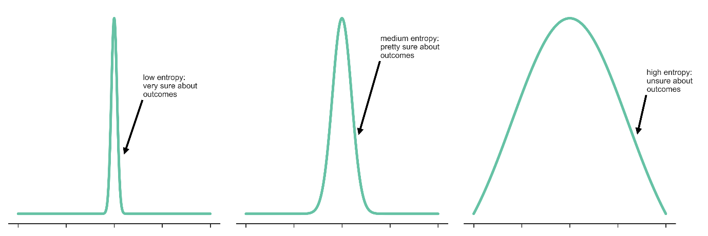
Entropy can be a somewhat tricky term, but I think this way of thinking about it is fairly intuitive: it’s just the amount you expect to be surprised by a given probability distribution. Some distributions are very tightly clustered around their average values, and so they are very unsurprising, hence low entropy. The opposite of this are the so-called maximum-entropy distributions, which means every sample is maximally surprising.

An example entropy calculation: A coin is a maximum entropy system, because it's maximally unpredictable, you don't know if it's going to come up heads $h$ or tails $t$ $$H(coin) = -P(h)\log P(h) - P(t)\log P(t)$$ $$H(coin) = -0.5 * \log(0.5) - 0.5\log(0.5)$$ $$H(coin) \approx 0.3$$ Now imagine if we had an unfair coin that came up heads with a probability of 90%: $$H(coin) = -P(h)\log P(h) - P(t)\log P(t)$$ $$H(coin) = -0.9\log (0.9) - 0.1\log (0.1)$$ $$H(coin) \approx 0.14$$ So the more certain we are about an outcome, the lower the entropy!

Equipped with these ideas, we define an energy-like function $\mathbf{E}(T,S)$:

$$\red{\mathbf{Ε}(T,S)}\ \equiv \red{- \ln{P(T,S)}}$$

And this allows us to rewrite our free energy term F as (remember the $\mathbf{E}(T,S)$ is defined as the negative of the log above, so we get a positive in the end):

$$F\ = \purple{\int_{}^{}{\text{dT}\ q(T)\ \ln{q(T)\ \ }}} -\int_{}^{}{\text{dT}\ q(T)\red{\ln{P(T,S)}}}$$ $$F = \int_{}^{}{\text{dT}\ q\left( T \right)\red{\mathbf{E}\left( T,S \right)}} + \purple{\int_{}^{}{\text{dT}\ q\left( T \right)\ln{q\left( T \right)}}}$$

Now, if we look at this formula (check that you see this from above) it looks like it’s saying that ‘free energy’ is equal to an average (expected value) of the energy-like function, minus something that looks a little like a continuous version of the entropy⁹. This version of the formula is something you’ll hear Friston refer to often, because it’s analagous to the Helmholtz free energy from thermodynamics/statistical mechanics: $F = U-TS$. The Helmholtz free energy is defined as the difference between the internal energy $U$ and the entropy $S$ of the system, multiplied by the temperature $T$. Here the term ‘free energy’ acquires some physical sense, being the quantity of energy in our system that is available to do useful work. Here I’ve split the $+$ into two negatives to emphasise we have a potential energy minus the entropy.

$$F = \int_{}^{}{\text{dT}\ q\left( T \right) \mathbf{E}\left( T,S \right) } - \left( - \int_{}^{}{\text{dT}\ q \left( T \right)\ln{q\left( T \right)} } \right)$$

Having gone through all of the above, we can now state the FEP explicitly:

The Free Energy Principle states that a system in nonequilibrium steady state with its environment must minimise its free energy

We’ll need another few posts to unpack everything there, but at minimum we now know what the ‘free energy’ term is and why minimising it might be useful!

Conclusion, Summary, and Anki Cards

We motivated the Free Energy Principle with three big ideas about living organisms:

• Eye on the (causal) prize
  • Survival depends on you figuring out what causes your sense data, because that allows you to model your environment
• All Reality is Virtual Reality
  • Survival depends on interpreting noisy correlates of the causes you care about. You can’t see the causes directly
• Macro-pattern, micro-random
  • You are made of atoms doing lots of small, random things, which you must self-regulate to keep within a broader set of viable patterns

Additionally, we learned:

• We want to calculate the probability of our environment, given our sense data, but the integral is intractable
• We use approximate Bayesian inference to get around this
• The G-density is a probability density function that tells us how environmental states correlate with sensations: $P(T,S)$
• The R-density is an internal best guess by the organism about the state of the environment: $q(T)$
• Minimising the KL-Divergence lets us approximate the posterior
• Free energy is an upper bound on surprisal
• We can rewrite our free energy as an average energy minus an entropy term, which makes it look like the Helmholtz free energy

As an experiment in what Michael Nielsen and Andy Matuschak dub the Mnemonic Medium, I’ve made a small deck of Anki cards that complement this post. If you use them, they’ll make the tricky vocabulary we’ve developed here into something you have stored in your long-term memory for easy use. You can download them here

In the next post, we’ll take the background we developed here and build on it. We’ll take a deeper look at the R and G densities and some simplifying assumptions that allow us to write neat versions of them. The result will show the deep connection between the Free Energy Principle and Predictive Coding in the brain.

If something here doesn’t make sense, is clearly wrong, or got you interested, let me know here or on twitter @jnearestn If you don’t want to wait for the next post, The Free Energy Principle for Action and Perception: A Mathematical Review is the best place to start out on your own, and I owe it a great deal in helping write this post!

---

Special thanks to Gianluca for his detailed comments on drafts of this post

1. The good news is that the Jeremy Howard rule holds: even if all of the math seems difficult, it will look much simpler in code ↩

2. shoutout to the New York Times for going full 2020 and trying to ruin that too ↩

3. See for example Friston’s reaction to a bunch of quants in this article ↩

4. in fact, this multiplicity of disciplines seems to set off a percentage of people’s BS-detectors, sort of like when Deepak Chopra starts invoking Quantum Mechanics as an explanation for everything ↩

5. if you don’t like 37, just use whatever number you were told by the last person who pointed one of those COVID-screening-thermometer-guns at your head ↩

6. there is of course the question of ‘why expect 37 degrees in the first place, why not 800 and then you can survive through more possible states’, to which the quick answer is “evolution” and evolutionary niches” – something like: that temperature is the constraint that you, as a particular organism, are forced to satisfy because of the particular set of biochemical pathways you evolved to best fit into your environmental niche (which seems, at this point, to be Zoom Meetings, for some reason?) ↩

7. 9 year old Jared knew a killer font when he saw one ↩

8. watch this video by Aurelien Geron if you want a great intro to the KL-divergence ↩

9. as I’m writing this, I’m learning that this continuous analogy of the entropy is not actually well-defined. It’s called differential entropy, and Claude Shannon apparently just wrote it down, assuming it was correct (okay, now I feel less bad for making the same assumption). It took E.T Jaynes to write down a better version called the ‘Limiting Density of Discrete Points’, which - at minimum - is a worse name than ‘differential entropy’. I don’t know what effect the ill-definedness of continuous entropy has for the FEP, so that’s something to look into while I write part 2! ↩